上一篇文章,我们总结了三种线性模型,并使用它们解决了二分类以及多分类问题。这篇文章主要介绍怎样解决非线性问题。
Quadratic Hypothesis
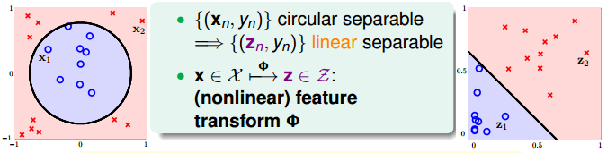
当数据非线性可分的时候,我们需要使用特征转换,将原来非线性空间上的特征转换到新的线性空间,然后再使用之前学过的线性模型进行分类。
特征转换如下:
$$\mathbf{x} \in \mathcal{X} \mathop{\rightarrow}^{\Phi} \mathbf{z} \in \mathcal{Z}
$$ 于是将非线性可分的样本 $\big\{ \big( \mathbf{x}_n,y_n \big) \big\} $ 转换为线性可分的样本 $\big\{ \big( \mathbf{z}_n,y_n \big) \big\} $
举一个例子说明:
下图中的样本 $\big\{ \big( \mathbf{x}_n,y_n \big) \big\} $ 是非线性可分的,但是可以使用圆将其分类。在使用特征变换 $$
\mathbf{z} = \Phi(\mathbf{x}) = (1, x_1^2, x_2^2)
$$ 之后,预测函数为 $$
h(\mathbf{x}) = \tilde{h}(\mathbf{z}) = \text{sign} \big( \tilde{\mathbf{w}}^T \Phi(\mathbf{x}) \big) = \text{sign} \big(
\tilde{w}_0 + \tilde{w}_1 x_{1}^{2} + \tilde{w}_2 x_{2}^{2} \big)
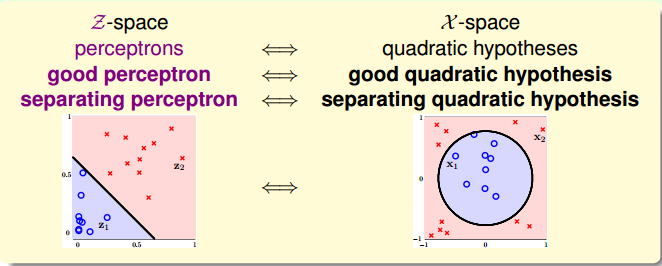
$$ 于是选择合适的参数,便可以使用直线将 $\mathbf{z}_n$ 进行分类,也就是使用圆将 $\mathbf{x}_n$ 进行分类。在这个例子中
$$
h(\mathbf{x}) = \tilde{h}(\mathbf{z}) = \text{sign} \big( \tilde{\mathbf{w}}^T \mathbf{z} \big) = \text{sign} \big(
0.6 + (-1) \cdot x_{1}^{2} + (-1) \cdot x_{2}^{2} \big) $$
当参数 $\tilde{\mathbf{w}}$ 取不同值的时候,在 $\mathbf{z}$ 域上看都是直线,但是在 $\mathbf{x}$ 域上看可以是圆、椭圆、双曲线等等不同的二次曲线。
Nonlinear Transform
可见,找到一个好的 Transform 方法,可以使得原始数据(不管是不是线性可分)分类的结果好。
因此,在遇到非线性可分的样本的时候,通常的做法是:
- 将原始数据进行转换 $\big\{ \big( \mathbf{x}_n,y_n \big) \big\} \mathop{\rightarrow}^{\Phi} \big\{ \big( \mathbf{z}_n,y_n \big) \big\}$
- 使用线性分类算法对转换后的数据 $\big\{ \big( \mathbf{z}_n,y_n \big) \big\}$ 进行分类
- 返回 $g(\mathbf{x}) = \text{sign} \big( \tilde{\mathbf{w}}^T \Phi(\mathbf{x}) \big)$
Price of Nonlinear Transform
当然,这样的做法也是有缺点的。
Computation/Storage Price
考虑 $Q$ 次多项式的特征转换![]()
可见,参数的个数是 $1 + \tilde{d} = O(Q^d)$,当 $Q$ 比较大时,时间复杂度以及空间复杂度都很大。
Model Complexity Price
模型的 VC dimension 是 $d_{\text{VC}} (mathcal{H}_{\Phi_Q}) \le 1 + \tilde{d}$ 可见当 $Q$ 比较大时,模型的 VC dimension 也很大。由此带来的问题是,可能会
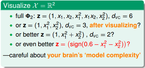
Danger of Visual Choices
还有一个问题是,在选择转化函数 $\Phi$ 的时候,可能加入了自己的脑力计算成果,这是不好的。
Structured Hypothesis Sets
Structured Hypothesis Sets
下面,我们讨论一下从 $\mathbf{x}$ 域到 $\mathbf{z}$ 域的多项式变换。
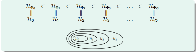
可见不同阶次构成的 hypothesis 有如下关系
$$ \mathcal{H}_0 \subset \mathcal{H}_1 \subset \mathcal{H}_2 \subset \cdots \subset \mathcal{H}_Q
$$ 对于 VC dimension 有
$$
d_{\text{VC}}(\mathcal{H}_0) \leq d_{\text{VC}}(\mathcal{H}_1) \leq d_{\text{VC}}(\mathcal{H}_2) \leq \cdots \leq d_{\text{VC}}(\mathcal{H}_Q)
$$ 对于 $E_{\text{in}}$ 有
$$ E_{\text{in}}(g_0) \geq E_{\text{in}}(g_1) \geq E_{\text{in}}(g_2) \geq \cdots \geq E_{\text{in}}(g_Q)$$
我们把这种结构叫做 Structured Hypothesis Sets。
Linear Model First
根据以前介绍过的学习曲线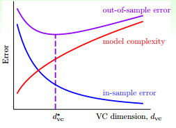
可以看出,当多项式的阶数增大时,$d_{\text{VC}}$ 变大,$E_{\text{in}}$ 变小,但是 model complexity 会变大。因此,需要选取合适的阶数使得 $E_{\text{out}}$ 较小。
一般的做法是,从一阶的 hypothesis 开始,如果 $E_{\text{in}}$ 足够小,就选择一阶,否则逐渐增加阶数,直到满足要求为止。